|
<< Click to Display Table of Contents >> Effect of the by-pass diodes |
  
|
|
<< Click to Display Table of Contents >> Effect of the by-pass diodes |
|
Hypothesis
Let's consider row arrangement systems only (sheds or trackers). In this case when one row puts its shade on the next one, the bottom cell row is primarily shaded.
Let's call sub-module the set of cells protected by one by-pass diode. In most modules (60 or 72 cells), there are 3 by-pass diodes and therefore 3 "sub-modules", usually disposed in length within the module.
Let's suppose that the modules are disposed in landscape, and all modules of the bottom row belong to the same string.
It is a common belief that with the mutual shadings, when the bottom sub-module (or even the bottom cells row) is shaded, the by-pass diodes will limit the electrical loss to the sub-module row, i.e. the string electrical production will remain 2/3 of the normal production.
This is not true ! When the bottom cells row is shaded, the full string becomes inactive for the beam component !
Consequences on the Electrical Shading loss calculations
| - | With the "Unlimited sheds" option, the width of the full string should be considered. As function of the profile angle, when the shade begins there is a transition corresponding to the width of one cell (half the cell shaded means half the current), and then the shading factor is full for this string. |
| - | With the calculation "according to strings" in the 3D model, this means that with row systems the Fraction for electrical loss should always be set to 100%. As soon as a part of the rectangle-string is shaded, the electrical yield is lost. |
| - | With the "Module Layout" model, the calculation is done correctly. |
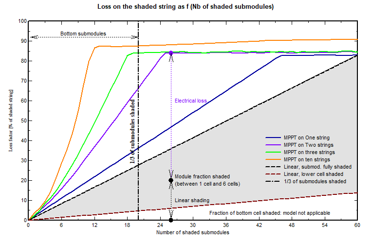
This graph presents the shading loss percentage for the full string, as a function of the number of shaded sub-modules.
This loss is dependent on the number of strings connected to the MPPT inverter input.
We can observe that when the MPPT input acts on one only string, the electrical shading loss is rather limited.
But as soon as you have 3 strings, when 1/3 of the submodules are shaded the loss (for beam) is total. Only the production corresponding to the diffuse is remaining.
This corresponds to a shading situation of this kind: only the bottom sub-modules are shaded:

We will try to understand this by observing the corresponding I/V curves, as calculated by the Module Layout model.
When we have one only string on the inverter input, the Maximum Power corresponds to the Pmpp of the unshaded sub-modules I/V curves. This means that if we have 1/3 of shaded sub-modules, the shaded Pmpp will be 1/3 of the normal Pmpp.
However this is not quite true because for each shaded submodule, the by-pass diode is activated, and leads to a voltage drop, therefore a Power loss. On the graph below, the blue characteristics corresponds to the 40 unshaded submodules, and the resultant shows the voltage drop.
On the graph above, this loss in diodes explains the gap between the MPPT loss factor (blue line) and the Linear, fully shaded straight line.
NB1: If the shaded Vmpp is lower than the minimum voltage of the inverter (VmppMin), then the operating point will be on the intersection of this voltage and the I/V curve: the electrical loss will very quickly rise to the maximum loss, up to the diffuse contribution, loosing the advantage of the 1-string per MPPT configuration. For this advantage, we should have an inverter accepting a very large voltage range.
NB2: This situation is also valid when several strings on one MPPT input are subject to the same shading situation. On the graph below, this would correspond to several identical strings added in current to this one. Therefore it may be interesting to connect all the strings of a same inverter to a same row (identically shaded) in the tables. This allows to concentrate the shading losses on one only MPPT, and let the other ones undisturbed.
This is only feasible when you have string inverters with 2 or 3 strings per MPPT, otherwise the string connection lengths may become prohibitive.
The Automatic Strings-Modules attribution tool allows this configuration: this is the option "Same row per MPPT".


On the top graph, we observe that for 3 strings the shading loss is already maximum when we have 1/3 of shaded sub-modules.
This corresponds to the following I/V curves: the first string partially shaded is identical to the previous one. But the 2 unshaded strings modify the resultant curve, and especially the Maximum power point: now the MPP imposes the voltage to all strings connected in parallel, and the operating point on the shaded string corresponds to the residual diffuse contribution.
This is the explanation of the affirmation above: the string contribution for the beam component is completely inactive !
NB: With this situation we are no more sensitive to the limitation with the VmppMin of the inverter.


On the top graph, the increasing parts of the curves correspond to the situation when the first MPP is higher than the secondary MPP due to the diffuse contribution. The plateau begins when the maximum is on the diffuse part (see the graph just above).
In this situation, we observe that with the 2-strings configuration we have still some contribution of the beam.
This graph was established for a 15% diffuse contribution. When the beam contribution decreases, the situation is improving and the curves move to the right.
The grey region corresponds to the linear shaded fraction: the bottom line represents the linear shadings when the bottom cell is shaded (1/6 of the full module). The upper dotted line is the situation when each concerned module is fully shaded. The shading loss - calculated from the I/V curves - represents the sum of the linear loss (effective shaded fraction of each sub-module) and the electrical loss is the complement. The electrical loss is maximal when only the bottom cell is shaded.
In PVsyst, you can get this diagram in the option "Tools > Electrical behavious of PV arrays > Array with shaded cells > By-pass diode effect".