|
<< Click to Display Table of Contents >> Electrical shadings: partition model |
  
|
|
<< Click to Display Table of Contents >> Electrical shadings: partition model |
|
The partition model for electrical shadings is an approximation that allows to compute electrical shading losses faster than with the detailed "Module Layout" mode. This approach works best in regular row-based systems.
This page describes the definition and implementation of the partition model. For guidelines on partitioning see this page.
General definition
The partition model is based on the observation that shading even a single PV cell may cause important mismatch losses, often leading to losing the power of a whole string of modules.
On each PV table in the 3D scene, one defines rectangles called partitions, each of these representing an area that may be impacted electrically by a single shade. When any of these partitions is sufficiently shaded, it is considered inactive (as far as the direct irradiance component is concerned). This electrically shaded partition is colored in yellow in the 3D scene animations.
The electrical loss on the beam component is calculated as the difference between the electrically shaded area, i.e. the yellow rectangular partitions, and the “linearly” shaded surfaces, shown in grey.
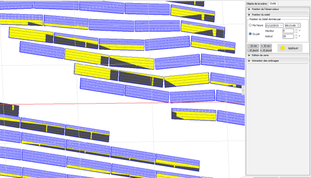
Figure 1: partitions with any amount of shading will be shown in yellow in the 3D scene animations.
The partition model is also called "according to module strings" in PVsyst. It is the historical way of computing the electrical effects of partial shadings in PVsyst, and the only way up to version 5. The model has received several improvements since, including factors that try to better account for cases with very little shading.
This approach works best for regular row-based systems. Some factors allow to adjust results in the case of irregular shadings.
Procedure
•In the 3D scene, you have to define the "Partitioning" for each PV table or arrays of the scene.
•If the scene has several PV tables or arrays, you have the option of transferring this partition size definition to all other PV tables/arrays.
•When these definitions are complete, back in the general "Near shadings" window, you can choose "Use in simulation > According to Module strings" and define the "Fraction for electrical effect".
Further notes:
•A “module layout” variant can be used as reference to help set the “Fraction for electrical effect”.
•As for the linear shadings, you have the option of a fast calculation (i.e. from the interpolation in the shading factor table), or a Slow calculation, with the full calculation of the shading factor from the 3D scene at each step of the simulation (more accurate).
Model
The real effect of partial shadings on the electrical production of a PV field is non-linear, and depends on the interconnections between the modules. The only way to take into account the interconnections in PVsyst is the "Module Layout" tool, but despite that in some situations the simpler partition model may be applied.
To understand the limits and applicability of the partition approximation, a key point is the following diagram, showing the total shading loss factor (clear-sky) on a given string, as a function of the number of shaded sub-modules, as well as the number of strings in parallel on a same MPPT. This graph is fully explained in the page "Effect of the by-pass diodes".
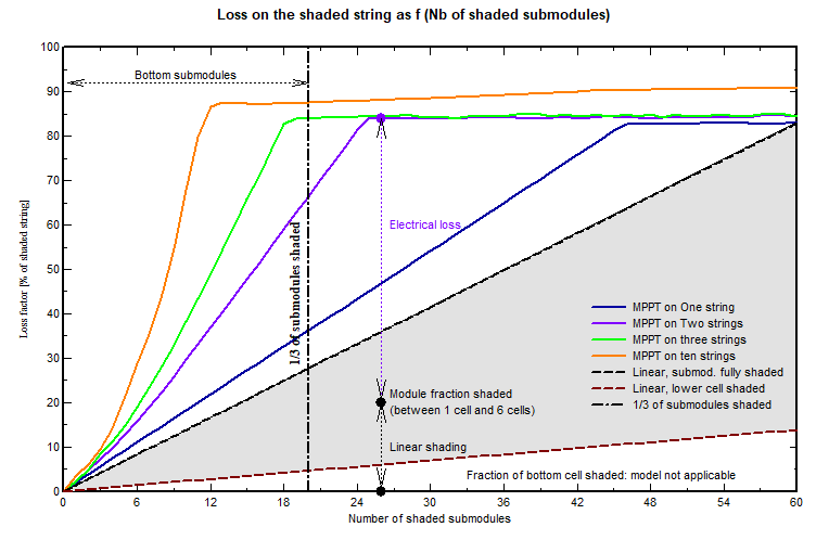
Figure 2: total shading loss factor as a function of the number of sub-modules shaded.
In the case of regular rows of tables or trackers, mutual shadings, when they are present, will affect at least the bottom sub-modules.
In the case of a longitudinal string with modules in the landscape configuration, the "bottom sub-modules" means 1/3 of the sub-modules. In Figure 2, this situation is shown by the vertical dot-dashed line. More important shadings may happen but less often, for lower profile angles: the mutual shadings will increase, gradually leading to the right of the graph.
In this landscape and low shade situation, i.e. moving vertically along the dot-dashed line, you can see that when there are 3 strings or more in parallel (green curve), the shading loss factor completely cancels the beam irradiance production. The loss reaches about 85% for clear-sky conditions. This justifies our hypothesis that in general, when part of the partition is shaded the production is almost completely lost. The case of 2 strings in parallel can be fairly well approximated by this case as well.
However, with only one string per MPPT (blue line), the curve shows that when 1/3 of sub-modules are shaded, the loss factor is only around 35%. To adapt the model to this situation, one can either increase the number of partitions, or define a "fraction for electrical effect" of the order of 42% (35% / 83% of beam). The former is to be preferred, since the fraction for electrical effect may also be used to account for irregular shading effects. The situation where only strings that have similar shadings are put in parallel on the same inverter input also falls in this case.
If the modules are in portrait, all the sub-modules are shaded at the same time, we are on the extremity of the curve, always fully shaded.
With twin half-cut cells modules in portrait, only half the current is lost when the bottom part is shaded, therefore the rectangle-string width should be the half-length of the module. The landscape case doesn’t differ from the previous discussion on standard modules in landscape.
Based on the observations of the previous discussion, the partition model aims at implementing the behavior shown in Figure 3. Over a partition, assuming regular row-based mutual shadings, the electrical shadings increase linearly with increasing linear shadings, until a cell width has been shaded. At this value the total shading loss reaches a plateau value. The direct irradiance shining on this partition is considered lost.
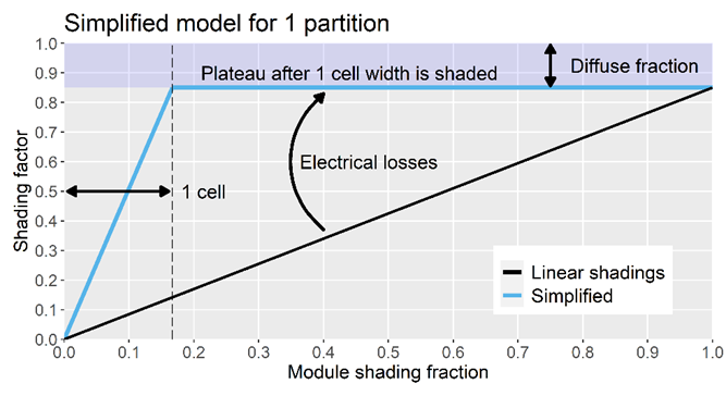
Figure 3: partition model definition
In practice, shadings are not necessarily regular. PVsyst therefore implements internally a decomposition of all partitions in 3 stripes shown in Figure 4:
•a central stripe, which if shaded, will force the maximum shading losses value on the partition,
•two one-cell-wide side stripes, on which the shading factor is considered proportional to the shaded area.
In regular situations this replicates the behavior of Figure 3.
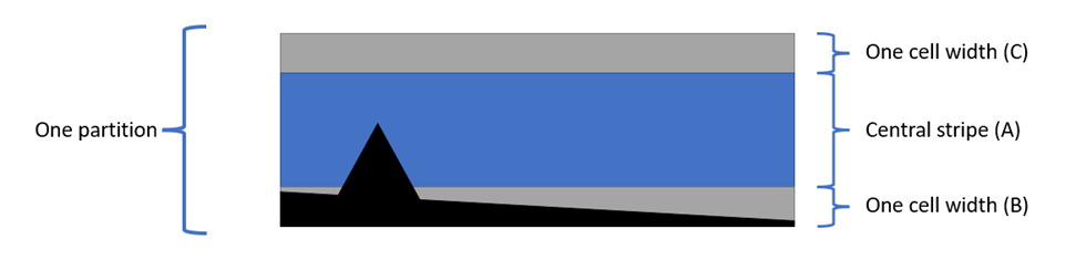
Figure 4: Model implementation with the central and side stripes. In the shading situation shown in black, the shading loss is maximum since the central stripe is shaded.
During the simulation, PVsyst may reduce the electrical shading loss from the partition model using a factor named "Fraction for electrical effect", that can be defined in the near shadings window. This allows to adjust the results to irregular shading situations, as discussed below.
The partition model also a special feature allowing to evaluate the shading effect of thin objects which only shade a part of one individual cell (like fences, HV lines above a PV array, etc). Any shading object defined as “thin object” will impact electrical shading losses separately from regular objects. A separate thin object fraction for electrical effect can also be defined in the near shadings window.
This kind of evaluation is currently not possible with the "Module Layout" tool.
We run extensive comparisons against the “Module Layout” model, which is considered most precise given row-based situations. Validations of the full PVsyst model against real systems have also been conducted in the past.
As the diffuse fraction grows, the real MPP of a shaded system may move beyond the scope studied in Figure A. For this reason validation against the “module layout” model is important as the latter captures better the MPP position in various conditions, as it is based on the combination of IV curves.
With irregular shadows, it is difficult to know whether a cell has been fully shaded or not, therefore the partition model is not really applicable. However, since whenever the central stripe is shaded the loss is maximum, we can consider that the calculation of the electrical factor according to the partitions gives generally an upper limit of the real shading loss.
During the simulation, PVsyst may reduce the electrical shading loss using a factor named "Fraction for electrical effect", to be defined in the near shadings window. The corresponding value of the "Fraction for electrical effect" is dependent on the shades distribution on the PV filed and the electrical array configuration. For a row-based arrangement (where the shades are very regular), it is near 100%. With more irregular shades like chimneys, far buildings, trees, it could be of the order of 60 to 80%, depending on the "regularity" of the shade (for example a diagonal shade could have a lower impact as it would concern modules better distributed in the PV array).
The Module Layout tool provides an accurate way of computing the real electrical losses in a much more extended range of situations. This may help for the evaluation of the "Fraction for electrical effect" in the case of irregular shadings.
A related example, in the case of a very large system, one may define a representative sub-system (for example corresponding to one central inverter), execute the simulation and evaluate the Electrical shading loss with both tools: Module Layout and partitions model; this will allow to evaluate the "Fraction for electrical effect" representative of your system.
Model history
The model did not account for bottom cell stripes. In other words, as soon as a partition was shaded, the shading loss was considered to be maximum. To mitigate the supplementary shading losses, a threshold at low linear shading values was implemented, that could cancel the electrical shading losses if there weren’t enough linear shadings.
Bottom cell stripe effects were implemented at the level of the whole scene. After the evaluation of linear shading factors, a general average shade height was computed. If that height was higher than half a cell width, the electrical shading losses went from zero to their maximum value.
This implementation tended to underestimate the electrical shading losses in the case of irregular shadings. Indeed the average shade height was often well below the actual shade on some of the most shaded partitions.