Effect of by-pass diodes and partial shading

Setting

Let's consider a row-based arrangement of PV tables (fixed tilt or trackers). In this case, whenever one row casts its shade on the next row, the bottom sub-modules, and in particular the bottom row of cells on the partially shaded table, are predominantly affected.

We call sub-module the set of cells protected by one by-pass diode. In most modules (60 or 72 cells), there are 3 by-pass diodes and therefore 3 "sub-modules", usually laid out in length within the module.

Let's suppose that the modules are laid out in landscape, and all modules of the bottom row belong to the same string.

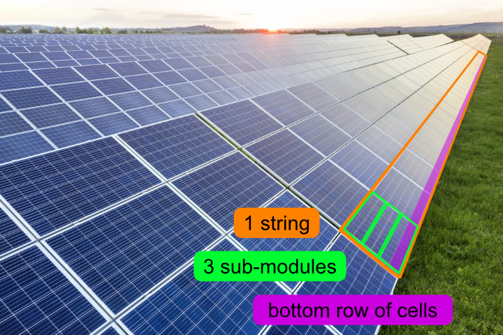
It is a common belief that with mutual shadings, when the bottom sub-module (or just the bottom cells row) is shaded, the by-pass diodes will limit the electrical loss to the sub-module row, i.e. the string electrical production will remain 2/3 of the normal production.

This is not necessarily true! When the bottom cells row is shaded, depending on the array interconnections, the beam contribution on the full string—instead of just 1/3 of it—may be jeopardized by the shadings!

To understand this, we will investigate the impact of shadings with a graph.

Shading loss as function of the number of shaded sub-modules

The following graph presents the shading loss percentage, normalized to the production of 1 unshaded string, on a clear-sky day, as a function of the number of shaded sub-modules. It includes the loss of irradiance and the electrical mismatch effects.

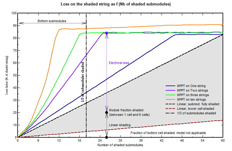
The shading loss (solid curves) is dependent on the number of strings connected to the MPPT inverter input (different colors).

We can observe that when the MPPT input has one only string (blue), the electrical shading loss is rather limited.

But as one increases the number of unshaded strings in parallel, the total shading losses increase. For 3 strings (2 unshaded and 1 shaded, green curve), when 1/3 of the submodules are shaded (dashed vertical line) the loss reaches about 85%. In other words, the direct irradiance contribution is lost in the shaded string. Only the production corresponding to the diffuse component (here about 15%) remains.

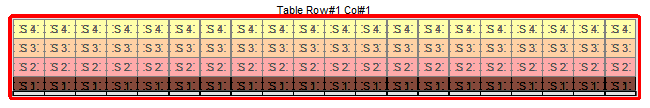
Schematically, this corresponds to a shading situation that looks as follows, where only the bottom sub-modules are shaded (here with 4 strings):

Note: this graph was obtained for clear sky conditions. In case of predominantly diffuse conditions, these conclusions may change.

In the next sections, we investigate this from another perspective: by observing the corresponding I/V curves, as calculated by the "Module layout" tool in PVsyst.

One only string on one MPPT

When there is only one string on the inverter input (or when all strings in this input are shaded in the exact same way), the maximum power corresponds approximately to the \(P_\textrm{MPP}\) of the unshaded sub-modules I/V curves. This means that if we shade 1/3 of the sub-modules, the shaded \(P_\textrm{MPP}\) will be 1/3 of the unshaded \(P_\textrm{MPP}\).

However this is not exactly true because for each shaded submodule, the by-pass diode is activated, and leads to a voltage drop, therefore a power loss. On the graph above, this loss in diodes explains the gap between the loss factor (blue line) and the straight line that counts the proportion of shaded sub-modules (black, dashed). In the graph below, the blue IV curve corresponds to the 40 unshaded submodules, and the green resultant shows the voltage drop.

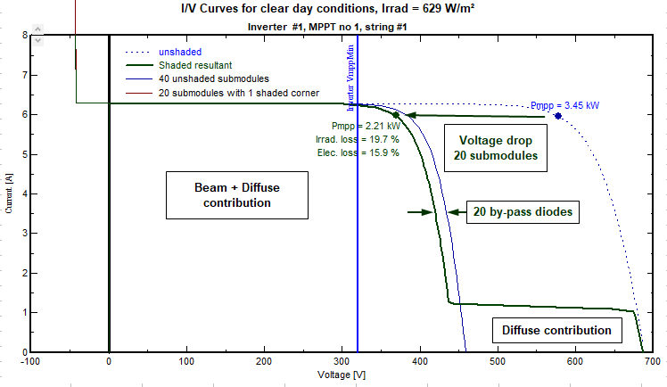
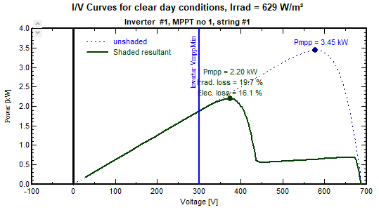
NB1: If the shaded \(V_\textrm{MPP}\) is lower than the minimum voltage of the inverter (\(V_\textrm{MPP,min}\), blue vertical line), then the operating point will be on the intersection of this voltage line and the I/V curve. This will generally displace the operating point towards higher voltages, where power drops quickly, up to the diffuse contribution part of the I/V-curve. The advantage of the 1-string per MPPT configuration can therefore be jeopardized by the inverter voltage range. To capitalize on the 1-string per MPPT situation, the inverter should accept a large voltage range.

NB2: This discussion is also valid when several strings on one MPPT input are subject to the same shading situation. On the graph below, this would correspond to several identical I/V caracteristics added—in current—to this one. Therefore it may be interesting to connect all the strings of a same inverter to a same row (identically shaded) over different tables. This allows to concentrate the shading losses on one only MPPT, and let the other ones undisturbed. This is only feasible when you have string inverters with 2 or 3 strings per MPPT, otherwise the string connection lengths may become prohibitive. In the module layout tool, the automatic Strings-Modules attribution tool allows this configuration: this is the option Same row per MPPT.

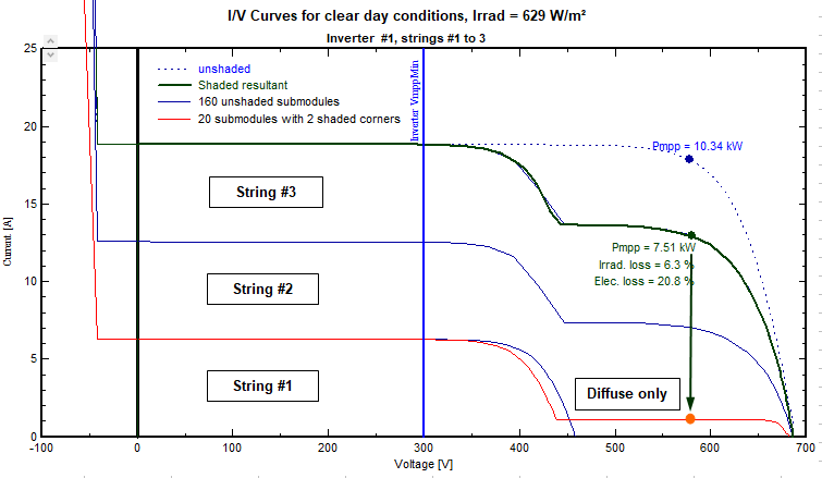
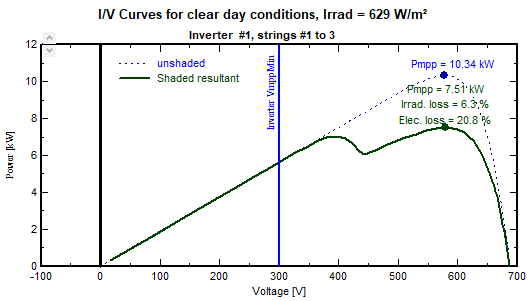
Three strings on one MPPT

On the top graph (shading loss as function of the number of shaded sub-modules), we observe that for 3 strings the shading loss is already maximum when only 1/3 of the sub-modules are partially shaded.

This corresponds to the following I/V curves: the first string partially shaded is identical to the previous one. But the 2 unshaded strings connected in parallel modify the resultant curve, and especially the maximum power point: now the MPP imposes the voltage to all strings connected in parallel, and the operating point on the shaded string corresponds to the residual diffuse contribution.

This is the explanation of the affirmation above: the direct irradiance contribution of the partially shaded string is naught !

*NB*: IN this situation, the MPP is not very sensitive to the \(V_\textrm{MPP,min}\) limitation of the inverter.

Interpretation of the Top graph

On the top graph (shading loss as function of the number of shaded sub-modules), the increasing parts of the curves correspond to the situation where the first MPP is higher than the secondary MPP due to the diffuse contribution. The plateau begins when the maximum is on the diffuse part (see the graph just above).

In this situation, we observe that with the 2-strings configuration (purple) some contribution of the beam subsists.

This graph was established for a 15% diffuse contribution. When the beam contribution decreases, the plateau of the diffuse contribution is reached more quickly. The loss, when normalized to the (decreasing) direct contribution, increases, but in fact the total loss factor may decrease.

The grey region corresponds to the linear shaded fraction: the bottom line represents the linear shadings when the bottom cell is shaded (1/6 of the full module). The upper dotted line is the situation when each concerned module is fully shaded. The shading loss—calculated from the I/V curves—represents the sum of the linear loss (effective shaded fraction of each sub-module) and the electrical loss is the complement. The electrical loss is maximal when only the bottom cell is shaded.

In PVsyst, you can get this diagram in the option Tools > Electrical behavious of PV arrays > Array with shaded cells > By-pass diode effect.