Calculation in the simulation
The Module Layout construction defines the exact position of each PV module in the 3D scene, and its electrical attribution to a given string in the system. The objective of the calculation within the simulation is to determine the electrical mismatch shading losses caused by partial shading of the beam irradiance component.
Calculation by MPPT input
During the simulation, the Module Layout calculation has to be performed at each time step, for each different MPPT input, i.e. for each set of strings connected in parallel, independently.
The basic data is the shade polygon calculated by the 3D scene on each table. This shade is applied on each submodule, which determines the "linear" shading factor for this submodule, as well as its electrical I/V curve.
Whatever the number of shaded cells within the submodule, the I/V curve of a shaded submodule remains quasi-identical. This is due to the fact that the current is driven by the cell with less irradiance, so that the I/V curve of the submodule is essentially the remaining production due to the unshaded diffuse irradiance. Therefore the submodule is the natural "unit" when calculating the I/V curve of a module or array. PVsyst distinguishes 4 typical submodule IV curves, depending on the number of submodule corners shaded.
I/V curve calculation
In a first step, the I/V curves of submodules in a string are added in voltage (i.e. Voltages of \(N_S\) shaded submodules + Voltage of \(N_U\) unshaded submodules for each current value). This gives a resultant I/V curve for the string.
In a second step, the currents of each string in parallel are added, leading to the resultant I/V curve of the MPPT input.
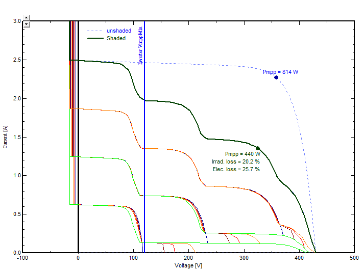
On this resultant curve, the inverter (MPPT) will "choose" the voltage corresponding to the Maximum Power Point. This will define the effective shaded power \(P_{\text{shaded}}\).
NB: in some cases the maximum voltage corresponding to \(P_{\text{shaded}}\) may be below the minimum voltage of the Inverter MPPT range (VmppMin). In this case PVsyst will choose the best value between the secondary MPP (corresponding to the diffuse) and the power at VmppMin.
Electrical Shading Factor
The global shading loss is \(P_{\text{mpp}}\) (of undisturbed array) \(- P_{\text{shaded}}\).
Now the shading loss is split into a "linear" shading loss contribution, evaluated from the geometrical shades on each submodule, and the "electrical" shading loss.
Therefore the final electrical loss is \(P_{\text{Elec}} = P_{\text{mpp}} - P_{\text{shaded}} - P_{\text{Linear}}\).
The shading factor on the beam component is finally \(P_{\text{Elec}} / (P_{\text{mpp}}\cdot \text{FracBeam}),\) where \(\text{FracBeam} = \text{Beam}/\text{Global}\) irradiances. Note that the global irradiance is understood as accounting for the shading of the diffuse.
Example
The graph below gives an example of a shaded sub-array of 4 strings. On the bottom string, 2/3 of submodules are shaded.
This kind of curve is available in the Module Layout window, page "I/V curve", for default clear sky conditions. It is not available for simulated time steps.
Impact of advanced parameters and thresholds
The module layout model is parametrized by several advanced parameters:
- Module Layout: Min. shade area to count as shaded : default value 0.024 m². When a small shade polygon covers a submodule without specifically covering a corner, the shade is neglected if below this area.
- Module Layout: Min. shading fact. for electrical calc. : default value 1%. If linear shadings are below this fraction for the string array, the electrical shadings are considered 0, i.e. \(P_{\text{Elec}} = 0\).
- Module Layout: Max. shading fact. for electrical calc. : default value 98%. Above this value the string array is considered fully shaded, i.e. \(P_{\text{Elec}} = 0\)
- Module Layout: Frac. bottom cell for no shading : default value 50%. When a shade covers only a fraction of a cell, the electrical loss behaves linearly with the fraction of cell shaded. Putting a threshold at 50% of a cell width in terms of the height of the shading polygon to activate the electrical shadings allows to model more closely the behavior of mutual shadings. Basically the linear increase over the cell width is approximated by a jump at 50% of the cell width.
